RASP-QS: Efficient and Confidential Query Services in the Cloud

1. Introduction

Hosting data query services in public clouds is an attractive solution for its great scalability and significant cost savings. However, data owners also have concerns on data privacy due to the lost control of the infrastructure. This demonstration shows a prototype for efficient and confidential range query services built on top of the random space perturbation (RASP) method. The RASP approach provides a privacy guarantee practical to the setting of cloud-based computing, while enabling much faster query processing compared to the encryption-based approach. This demonstration will allow users to more intuitively understand the technical merits of the RASP approach via interactive exploration of the visual interface.

Download: version 1.0

References:

- Zohreh Alavi, Lu Zhou, James Powers, and Keke Chen, "RASP-QS: Efficient and Confidential Query Services in the Cloud", International Conference on Very Large Databases (VLDB), Demonstration Session, 2014

- Huiqi Xu, Shumin Guo, and Keke Chen: "Building Confidential and Efficient Query Services in the Cloud with RASP Data Perturbation ", accepted by IEEE TKDE in Nov. 2012, appears in Volume 26, Issue 2, 2014

- Keke Chen, Ramakanth Kavuluru, Shumin Guo " RASP: Efficient Multidimensional Range Query on Attack-Resilient Encrypted Databases ", ACM Conference on Data and Application Security and Privacy (CODASPY), 2011

2. Install the demo system

You need to install the following items before you can run the demo system.

- The latest version Java

- Python 2.7 and numpy

After that, simply extract the downloaded zip file. The first time running the demo, you will need to configure the major paths: the python installation directory, the python code directory, and the working directory, with the “Config” button. The default setting works for Windows environments in normal cases. For linux, you will definitely need to change the setting.

3. Using the demo system

The current version of the demo system is a simple client-only visual interface to show

-        how the data is perturbed,

-        how the query is transformed,

-        and the result of two-stage query processing.

The visualization part uses our previously developed VISTA system for visual exploration of multidimensional datasets.

Sample Datasets

The target datasets are multi-dimensional numeric data. Each row in the data file should contain a comma separated data record. We have included three sample datasets in the demo package:

-        adult.d5.20k, which is derived from the Adult dataset in the UCI database  (http://archive.ics.uci.edu/ml/datasets/Adult) . It only contains 5 dimensions.

-        uniform.d5.100k and normal.d5.100k are two synthetic datasets, with multi-dimensional uniform and normal distributions, respectively. These two datasets are dense, and thus the labeled items might be overlapped by other items. Interactively explore the visualization to find the labeled items. Both have 5 dimensions.

Overview of the user interface

On the top side of the window are the dataset and query setup controls. From this area, you can select a dataset, generate perturbation parameter, perturb data, generate queries, and transform queries. When the datasets and query results are ready, the results will be visualized on the bottom two panels.

To test queries, you can choose to generate random queries and optionally tune it manually with the “Query” controls. Once the original query is composed, you can transform it and observe the transformed query that contains the Minimum Bounding Box (MBR) and the query matrix for each bound (the lower and upper bounds for each dimension).

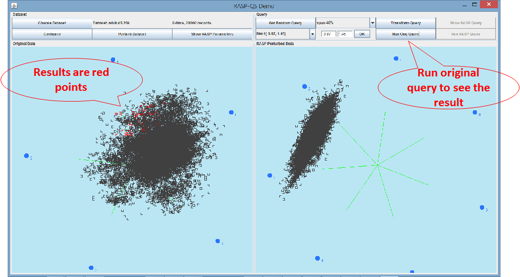
We do not include the index-supported query processing in this demo. Therefore, for large datasets it will take some time to process the query. The query result on the “Original Data” panel is highlighted with red points. Correspondingly, on the “RASP Perturbed Data” panel you can find these red points, but in the perturbed space. The “RASP” visualization also includes the blue points, which are the result of the first stage of RASP query processing. 

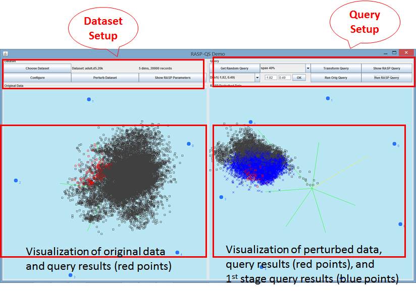
Figure 1: the UI overview

Detailed Operations with Examples

After choosing dataset, the dataset will be visualized automatically. The initial Python program is set to “C:/Python27/python”, the python code is in the subdirectory “./python/”of the current directory, and the working directory is set to “./tmp”. You will need to change them if your system setting is not like this, especially for Linux systems. Once the dataset is loaded, some buttons are enabled to allow further steps.

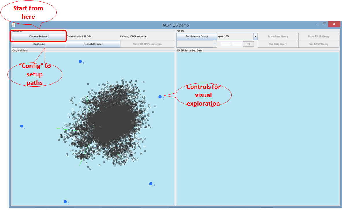
Figure 2. Visualization of the original dataset. The five blue dots are for dimensional parameter control. You can press on any one of them to change the weights of that dimension.

Click “Perturb Dataset” to generate perturbation matrix A, perturb the original data, and visualize the perturbed data. Click “Show RASP Parameters”, you will see the Matrix A.

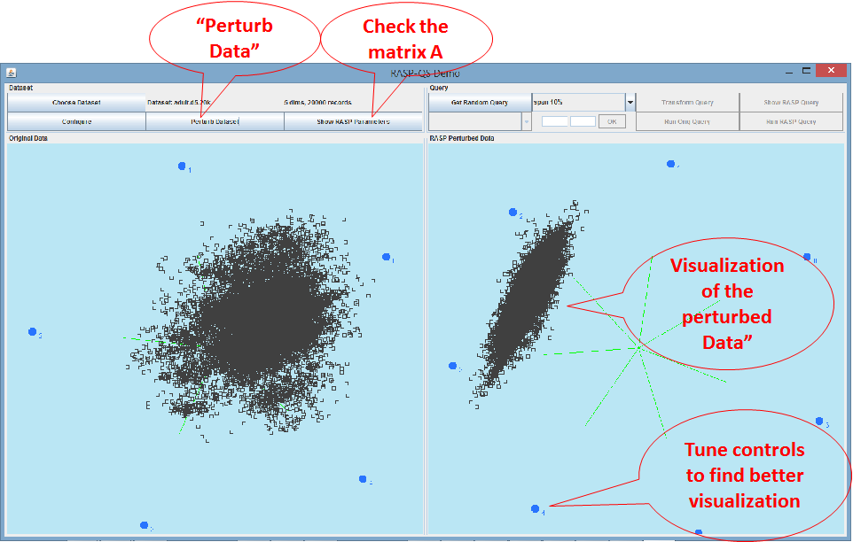
Figure 3. Perturb data, visualize the perturbed data, and check the matrix “A” for perturbation.

On “Query” control section, you can choose the span of the random query first. Due to the sparsity of the multidimensional space, larger spans will give you better chance to include some records in query results. Typically Spans >30% are good for higher dimensional datasets. By clicking “Get Random Query”, you can generate one random query for the original dataset. The result can be observed in the combobox. You can further tune each dimension by selecting it from the dropdown list, type in values, and click “OK”.

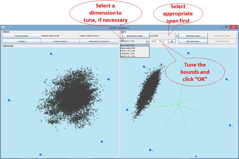
Figure 4. Generate a random range query for the original dataset

After you are done with editing the range. By clicking “Run Original Query”, you can see the result of the query are highlighted as red points on the left bottom panel. If you cannot see them, probably the result set contains 0 records, or it contains only a few points that are buried by other points. In the latter case, by tuning the visualization you can see them.

Figure 5. Visualization of the query results on the original dataset.

Click “Transform Query” to transform the query to the perturb space and then you can click the next button to observe the details of the transformed query. After that the “Run RASP Query” button should be enabled. Click it you will see the results are highlighted in blue (the 1^st stage result – the final result) and in red (the final result). Tune the visualization parameters to find the best result.

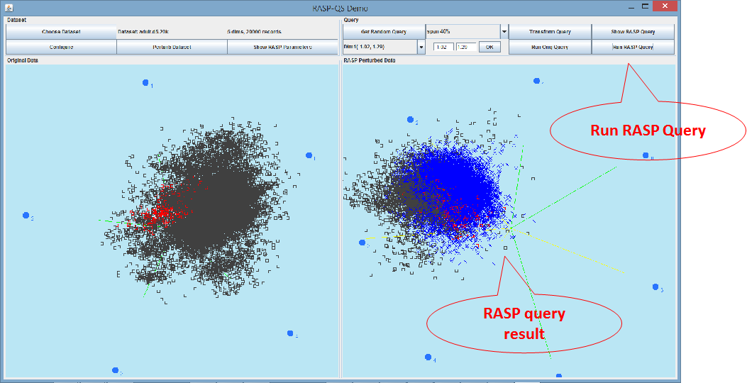
Figure 6. Visualization of the RASP query result in the perturbed space.